
Find the median of any list of numbers, along with the quartiles, interquartile range, and a complete step-by-step breakdown. Works for both odd and even data sets.
| Quantity | Value | Formula | Notes |
|---|
| Position | Sorted value | Group | Note |
|---|
| Metric | Value | Notes |
|---|
-
Select a citation style above. Click the citation text to select it all, then copy.
ADVERTISEMENT

Founder & CEO, Toolraxy
Faiq Ur Rahman is a web designer, digital product developer, and founder of Toolraxy, a growing platform of web-based calculators and utility tools. He specializes in building structured, user-friendly tools focused on health, finance, productivity, and everyday problem-solving.
User Ratings:
ADVERTISEMENT
ADVERTISEMENT
The median is the middle value of a data set after the numbers are sorted from smallest to largest. If the count is odd, it’s the single middle number. If the count is even, it’s the average of the two middle numbers. The National Institute of Standards and Technology defines the median as the 50th percentile, the value where half the observations sit below and half sit above.
Statisticians reach for the median when the data has a long tail or a few extreme values. Income and home prices are the classic examples. A handful of billionaires or mansions can pull the mean far above what most people experience. The median stays near the center because it only cares about position, not magnitude. That robustness is why government agencies and housing economists report median figures alongside averages, and why the UK’s Herefordshire council explains that median house prices give a “fairer result” than means when the distribution is skewed. The trade-off is that the median ignores the actual distances between values. Two data sets can share a median while looking completely different in spread.
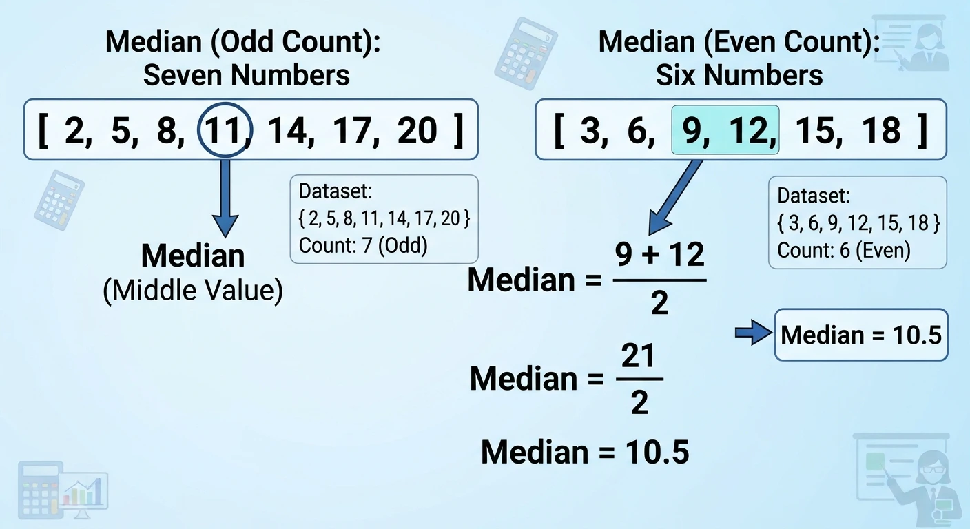
Sort the numbers from smallest to largest, count how many there are, and pick the middle position. If the count is odd, that position holds the median. If the count is even, average the two middle values. The calculator does the sorting and counting for you.
Paste or type your numbers into the data set box. Commas, spaces, semicolons, and new lines all act as separators.
Check the “Values detected” field. If the count doesn’t match what you expected, scan for a stray letter or a double separator that broke a number in two.
Set the decimal places for the display, from zero to six. The default is two.
Read the median from the large result at the top. The context line tells you whether the count is odd or even.
Look at the quartile tiles for Q1 and Q3, then check the IQR in the summary table.
Scroll to the step-by-step table to see the sorted list. The median row is highlighted, and the lower and upper halves are labeled.
If you need the arithmetic average instead of the middle value, the mean calculator uses the same input format and returns the sum divided by the count.
The median formula depends on whether the sorted count nn is odd or even. For an odd count, the median sits at position (n+1)÷2(n+1)÷2. For an even count, it’s the average of the values at positions n÷2n÷2 and (n÷2)+1(n÷2)+1.
Formula (even n): Median = (sorted[n ÷ 2] + sorted[(n ÷ 2) + 1]) ÷ 2

Formula (IQR):    IQR = Q3 − Q1
Quartiles split the sorted data into four parts. This calculator uses the exclusive method: Q1 is the median of the values below the median, and Q3 is the median of the values above it. The median itself is excluded when the count is odd. The Scribbr guide to interquartile range explains that the exclusive method is common for even-count data and tends to produce a wider IQR than the inclusive method. That’s a feature, not a bug: the exclusive IQR captures more of the middle spread.
A courier logs ten delivery times: 14, 18, 22, 25, 29, 31, 35, 38, 42, and 47 minutes. The count is even, so the median is the average of the fifth and sixth sorted values: 29 and 31. That gives 30 minutes.
The lower half is 14, 18, 22, 25, and 29. Its median, Q1, is 22. The upper half is 31, 35, 38, 42, and 47. Its median, Q3, is 38. The interquartile range is 38 − 22 = 16 minutes. That means the middle 50% of deliveries landed within a 16-minute window. The mean comes out to 301 ÷ 10 = 30.1 minutes, almost identical to the median because these delivery times are fairly symmetric. If one delivery had taken 120 minutes instead of 47, the mean would jump to 37.4 while the median would stay at 30. That’s the outlier resistance in action. The range runs from 14 to 47, a spread of 33 minutes.
The median is the middle value after sorting; the mean is the sum divided by the count. The median ignores how far the extremes sit from the center, while the mean uses every value, so one extreme number can pull the mean far away.
| Dimension | Median vs mean |
|---|---|
| Calculation | Median: sort and pick the middle (or average two middles). Mean: add all values and divide by the count. |
| Outlier sensitivity | Median barely moves when one value changes; mean can swing sharply. |
| Skewed data | Median represents the typical case better; mean gets pulled toward the long tail. |
| Symmetric data | Both land close together; the mean uses more information. |
| Small data sets | Median is stable but coarse; mean can be distorted by a single entry. |
| What this calculator reports | Median is the headline result; mean appears in the summary table for comparison. |
The median wins when the data has a long tail. Home prices and household incomes are the textbook cases: a few ultra-expensive sales can drag the mean well above what most buyers actually pay, while the median stays near the middle transaction. The IMF’s housing price analysis notes that because house price distributions are positively skewed, the median is typically used instead of the mean. The mean wins when every value should count equally and the distribution is balanced. Test scores, measurement averages, and temperatures usually fall into that bucket. A geometric mean calculator is a different alternative for growth rates and ratios, where multiplying values makes more sense than adding them.
The median is the middle value of a sorted data set. Half the values sit below it and half sit above it. If the count is even, it’s the average of the two middle values.
Sort the numbers from smallest to largest, count them, and pick the middle position. For an even count, average the two middle numbers. The calculator does this automatically and shows the sorted list.
The median is the middle value after sorting; the mean is the sum divided by the count. The median resists outliers, while the mean gets pulled by extreme values. Income and home prices are usually reported as medians for that reason.
In everyday speech, “average” often means the mean. The median is a different type of average. Statisticians call both measures of central tendency, but they answer different questions. The arithmetic mean calculator handles the sum-divided-by-count version.
Skewed data has a long tail on one side. The mean gets pulled toward that tail, sometimes far from what most values look like. The median only cares about the middle position, so it stays near the center.
The IQR is the difference between the third quartile and the first quartile: IQR = Q3 − Q1. It measures the spread of the middle 50% of the data and ignores the tails.
The exclusive method removes the median before splitting the data into halves. Q1 is the median of the lower half and Q3 is the median of the upper half. This calculator uses the exclusive method.
Yes. When the count is even and the two middle values differ, their average can land between them. For 29 and 31, the median is 30. For 10 and 15, the median is 12.5.
Sort the data and average the two middle values. For ten values, average the fifth and sixth. For eight values, average the fourth and fifth.
Use the median when the data has extreme values or a long tail. Home prices, incomes, and wait times are common cases. Use the mean when every value should count equally and the distribution is roughly symmetric.
Yes. The sorting step handles negatives correctly, and the median can be negative if the middle values are below zero. Temperature data is a common case.
The parser splits on spaces, commas, and semicolons, then converts each token to a number. Tokens that don’t convert are ignored. The verdict line tells you how many entries were skipped.
The National Institute of Standards and Technology’s percentile definitions define the median as the 50th percentile, the value where at most half the measurements are below and half are above.
Scribbr’s guide to the interquartile range explains the exclusive and inclusive quartile methods and notes that the exclusive method is common for even-count data.
The UK Herefordshire Council’s explanation of median house prices and earnings describes why the median gives a fairer picture than the mean when extreme values are present.
The International Monetary Fund’s housing price analysis notes that house price distributions are positively skewed and that the median is typically used instead of the mean.
The U.S. Environmental Protection Agency’s guidance on box plots documents the 1.5 × IQR fence rule for identifying potential outliers.
American Default’s glossary entry on median home price provides the example of how a single $10 million sale skews the mean but barely moves the median.
Arithmetic mean calculator – computes the sum-divided-by-count average so you can compare it with the median.
Median calculator – runs the sorted-middle calculation so you can compare it with the mean.
GPA calculator – handles the credit-hour weighting that a plain arithmetic mean ignores.
This calculator is an educational and utility tool. It performs the median and quartile calculations described on this page, but it does not provide statistical consulting, financial advice, medical advice, or any other professional service. If you’re using a median to make a decision that carries financial, health, or safety consequences, confirm the result with a qualified professional who can review the data and its assumptions.
ADVERTISEMENT
ADVERTISEMENT